Bachelor thesis: Reinforcement Learning vs Classical Control for racing a TurtleBot 4
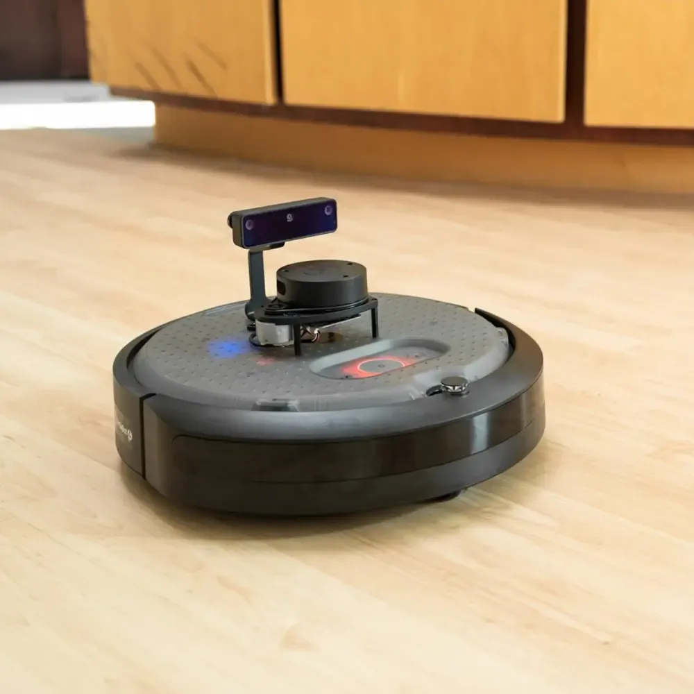
This post is about my Bachelor’s thesis at the Universidad de Alcalá, presented in July 2026: trajectory planning and control for autonomous racing vehicles using Reinforcement Learning, applied to the TurtleBot 4 Lite. I developed it during my research internship at the RobeSafe Group.
The question behind it is simple. When the goal is to drive a circuit as fast as possible, is Reinforcement Learning (RL) a real improvement over classical controllers? And can an RL agent discover a good racing line on its own?
The short version:
- In simulation, the RL agent set the fastest lap on the circuit I used for the comparison, but by a small margin over classical controllers following an optimized racing line.
- It paid for that speed with a larger tracking error and a rougher ride.
- On the real robot, lap times were almost identical for the four controllers, and the RL agent was the least precise one. The sim-to-real gap was the limiting factor.
1. Introduction and objectives
The main objective was to analyze to what extent RL improves on classical controllers in autonomous racing. In practice, that meant three things:
- Creating an RL agent that can follow trajectories in the shortest time possible.
- Comparing it against classical control algorithms, both in a simulator and on the real robot.
- Drawing conclusions about the performance and robustness of each approach.
To get there, the work is built on three pillars:
- Planning: turning reference tracks into geometric racing lines designed to maximize sustained speed and minimize lap time.
- Classical control: making Pure Pursuit, LQR and MPC follow those precomputed lines and measuring their tracking accuracy and lap times.
- Reinforcement Learning: training a DDPG agent and checking whether it can learn to drive efficiently and find the ideal line by itself, then comparing the path it discovers with the one calculated mathematically.
2. System architecture
2.1 General architecture
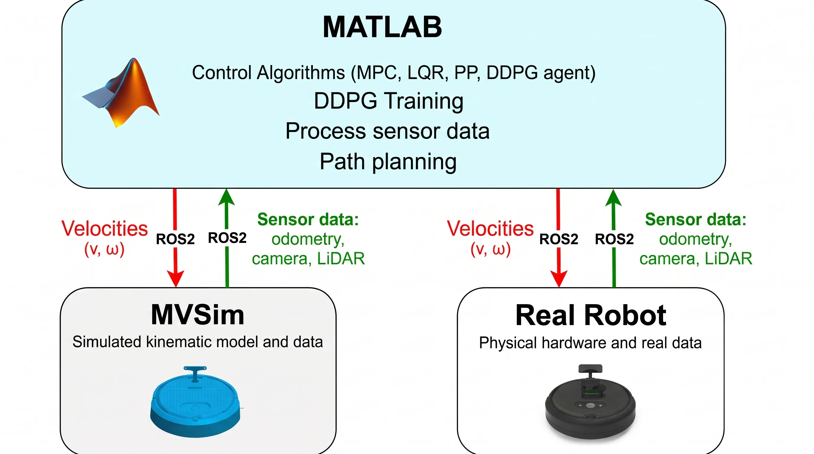
MATLAB is the brain of the system. It runs the control algorithms (MPC, LQR, Pure Pursuit and the DDPG agent), trains the agent, processes the sensor data and plans the trajectories.
It talks over ROS 2 with one of two “bodies”: the MVSim simulator, which provides simulated data and a kinematic model of the robot, or the real TurtleBot 4. In both cases the loop is the same. MATLAB sends linear and angular velocities (v, ω) calculated by the different algorithms, and receives odometry, camera and LiDAR data from the robot.
2.2 Circuit modeling
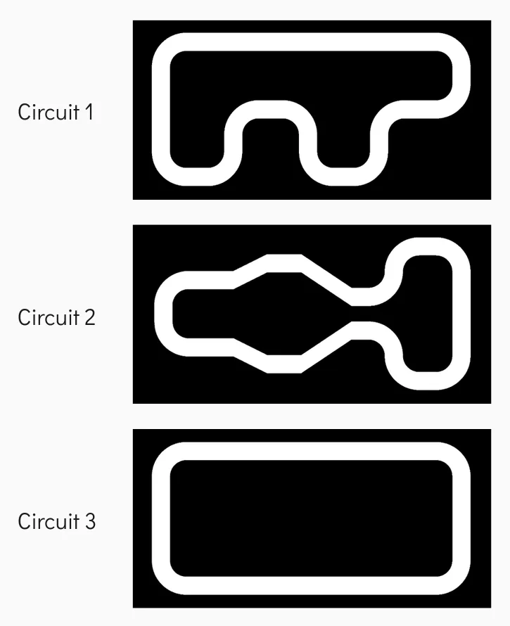
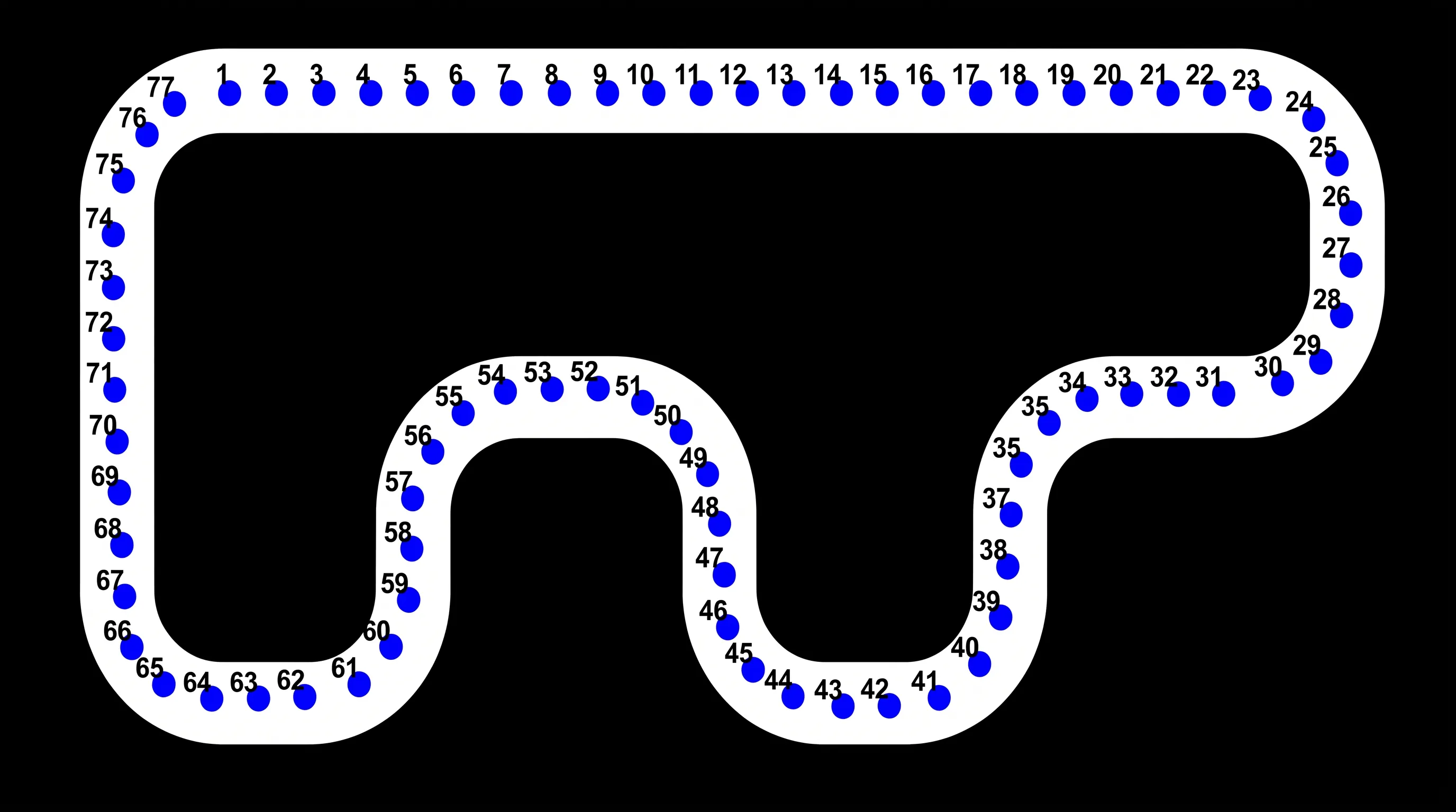
I designed three circuits of increasing complexity:
- Drawn in Paint and exported as PNG images.
- Track width of 0.80 m.
- Dimensions of 16 m × 8 m.
3. Trajectory planning
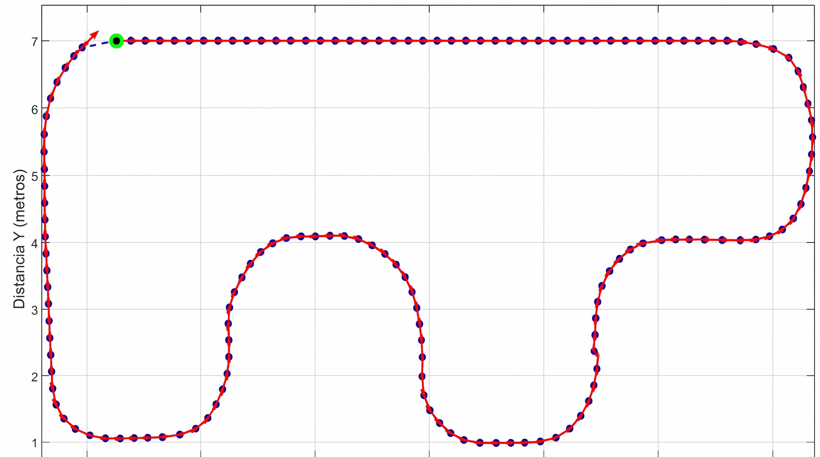
Planning has two steps: generate a set of reference coordinates that define the circuit (the waypoints), and join them into a smooth trajectory.
3.1 Waypoint generation
I used two alternatives.
Equispaced waypoints. I teleoperate the robot from my computer, and a waypoint is saved every 0.25 meters.
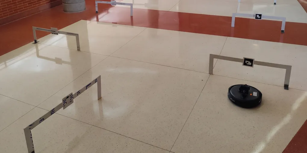
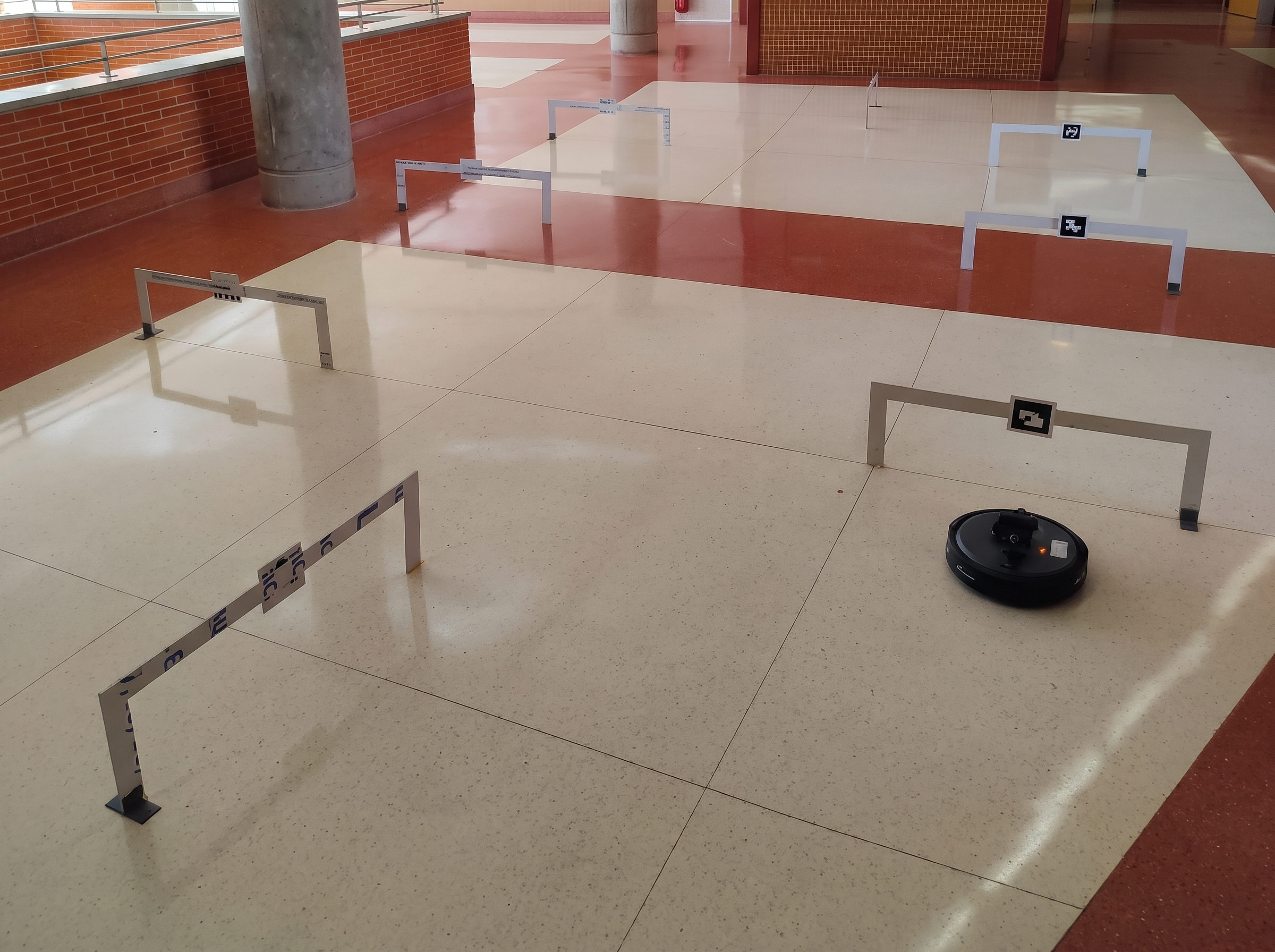
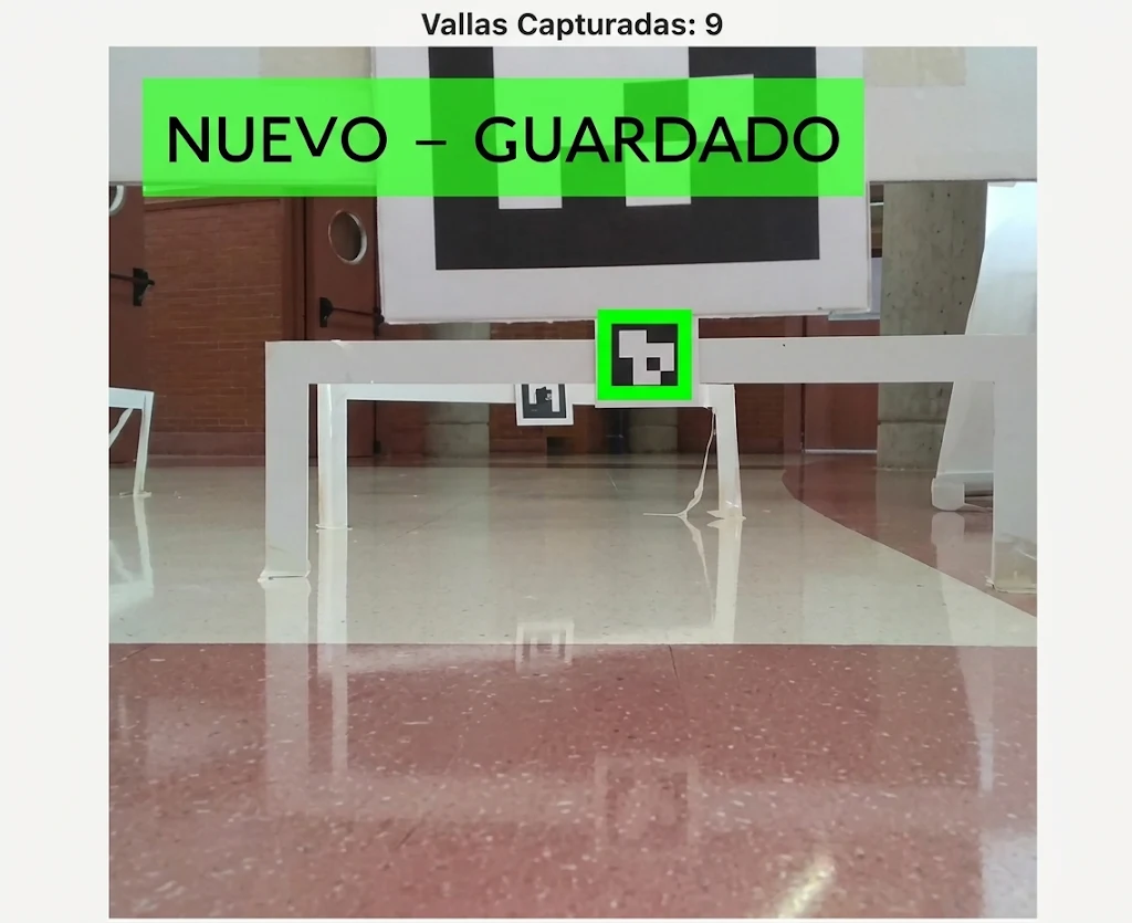
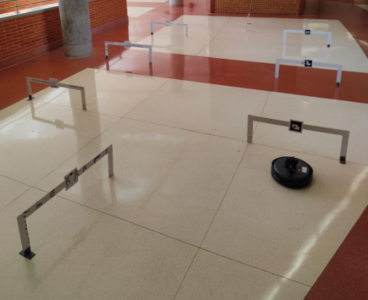
ArUco markers. I place small fences carrying ArUco markers, ordered chronologically by ID. While I teleoperate the robot, it detects the markers, and one waypoint is saved for each marker detected. This makes it possible to define a circuit on a real floor.
3.2 Trajectory generation
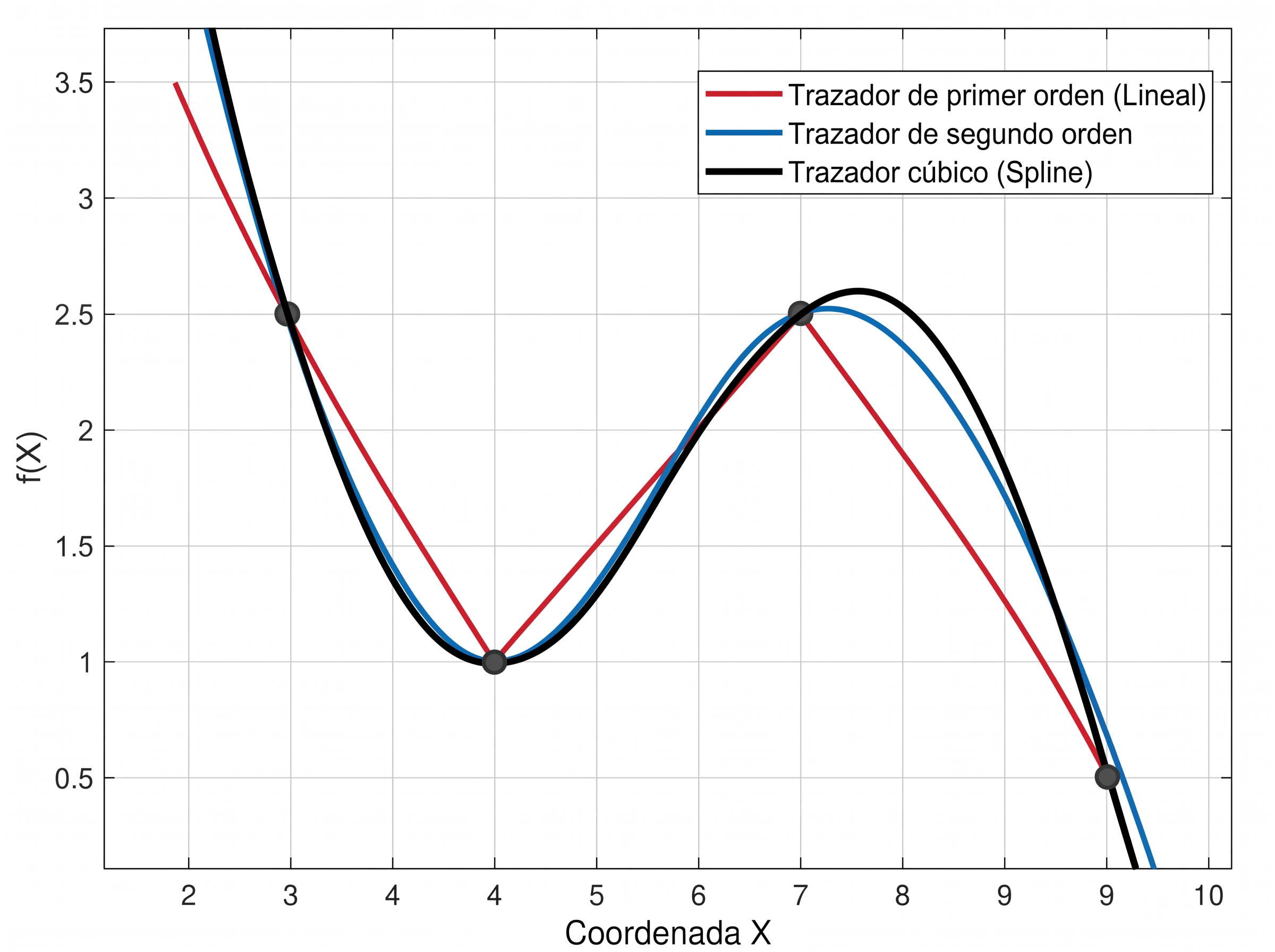
To join the waypoints I use splines. A spline guarantees that both the orientation and the curvature are identical when entering and leaving each point, so the resulting path is smooth and the robot can follow it without abrupt changes.
3.3 Trajectory optimization
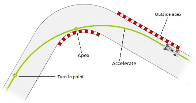
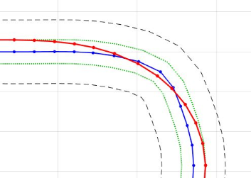
The centerline is not the fastest way around a circuit. The goal here is to find the racing line: the path that maximizes the speed through corners, to minimize lap time.
The maximum speed the robot can sustain at each point depends on the curvature κ(s) of the path:
v_max(s) = sqrt( K_max / |κ(s)| )The flatter the curve, the faster the robot can go. So the optimization minimizes the global curvature of the reference centerline by moving the points sideways, always within a safety limit (±15 cm) so that the robot never touches the walls.
4. Control methods
The core of the thesis is a comparison between two families of controllers:
- Classical algorithms:
- Pure Pursuit steers the robot towards a look-ahead point on the path.
- LQR is a state-feedback controller obtained by minimizing a quadratic cost on the tracking error and the control effort.
- MPC solves an optimization over a short horizon using a model of the robot (unicycle), applies the first command and repeats.
- Reinforcement Learning: a DDPG agent that learns its own control policy by interacting with the environment.
Both Pure Pursuit and MPC algorithms use a lookahead (horizon) of 10 waypoints ahead. This means that they use the next 10 waypoints (approximately 2.5 meters) to anticipate what’s coming and take the curves smoothly. A good analogy is how humans drive: we always look several meters ahead of our car to anticipate or predict the road; MPC and Pure Puresuit work the same way.
5. Control and training of the RL agent
5.1 Reinforcement Learning
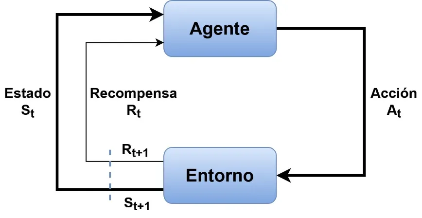
RL is a loop between an agent and an environment. At each step the agent observes a state, takes an action, and receives a reward. Here:
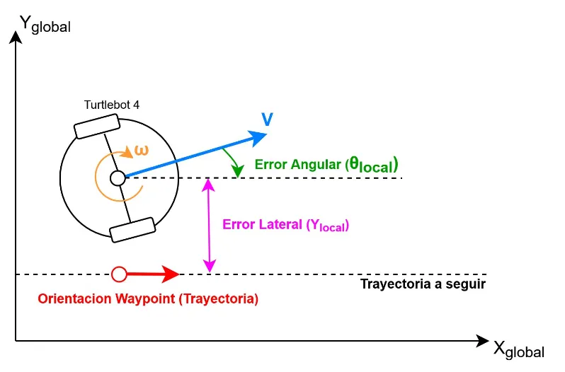
- State: the robot’s local view, meaning its angular error and its lateral error with respect to the trajectory (current waypoint).
- Action: linear and angular velocity.
- Reward: a mathematical signal that rewards maximizing speed and penalizes deviations.
5.2 DDPG: actor-critic architecture
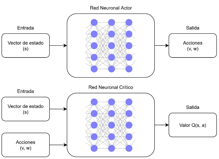
DDPG (Deep Deterministic Policy Gradient) uses two neural networks. The actor takes the state vector and outputs the actions (v, ω). The critic takes the state and the actions, and outputs the value Q(s, a), an estimate of how good that action is in that state. The critic’s feedback is what teaches the actor to output better actions.
TODO: add the size of the networks and the main hyperparameters.
5.3 DDPG: observation space
The state vector gives the agent a local perspective with only two values: the lateral error with respect to the current waypoint, and the angular error between the robot and the trajectory. The agent does not see the whole map, it only sees the next (current) waypoint.
5.4 DDPG: reward function
At every step the agent gets a dense reward:
r = v · ( |cos(θ_local)| − |sin(θ_local)| − |y_local| )Here v is the speed, θ_local is the angular error and y_local is the lateral error. The term in parentheses is largest when the robot points along the path and stays centered (close to 1), so going fast only pays off if the robot keeps its heading and position. In other words, the agent knows that the higher the speed, the higher the reward. But high speed doesn’t mean anything if the lateral error and angular error are huge. Consequently, the agent must find the right trade-off between high speed and those errors to maximize the reward at each step. Lately we will see that the agent found out that it prioritizes higher speed rather than lateral errors, because, in the end, the main purpose of this work was finding the fastest way to complete a lap within the track limits.
Additionally, there are also two sparse rewards that mark the end of an episode:
- Leaving the track (−20): if the lateral error exceeds the physical safety limit of the track (0.23 m), the agent is penalized and the episode ends.
- Finishing the circuit (+200): if the agent reaches the last waypoint of the sector or the circuit, it gets a bonus, because it has achieved the main goal: completing the whole route.
5.5 DDPG: training strategy
The training went through two stages: the whole circuit and task randomization.
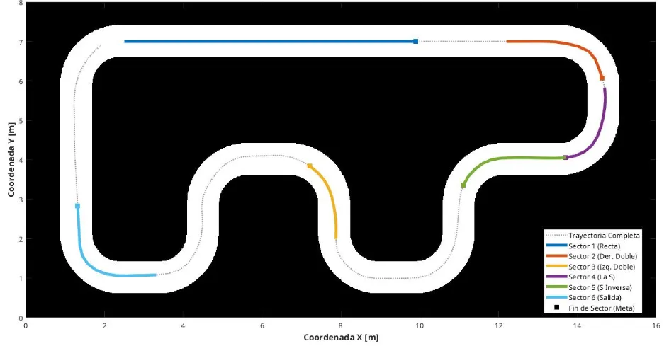
Training with the whole circuit was not ideal because the observation state was tremendously large (too many waypoints). No beginner learns driving at the Nordschleife… you must start at the bottom. For that I used the technique called task randomization, which consists of training the agent with easy random tasks instead of bigger and more complex ones (whole circuit). I split the main circuit into six sectors: a straight, a double right, a double left, a chicane, an inverse chicane and the exit (curve+straight). Alternating the sectors was used to fight catastrophic forgetting, which happens when an agent forgets how to drive a sector it already learned once it practices another one. By randomizing the sectors, the agent learnt how to drive on a straight or a chicane at the same time from zero. It didn’t know which sector would come next, as they all had the same probability of appearing. With this, the agent had to change its network weights to try to adapt to all those sectors at once, solving the overfitting and catastrophic forgetting problem.
5.6 DDPG: training convergence
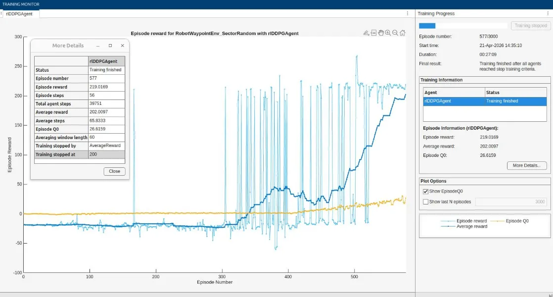
The training stopped by itself when the average reward over the last 60 episodes reached 200, meaning the last 60 episodes reached the finish line of that trained sector (+200 bonus reward). That happened at episode 577 (out of a maximum of 3000), after about 39,700 steps and roughly 27 minutes of training in MATLAB.
The learning curve is clear. For about the first 300 episodes the average reward stayed around −20, the penalty for leaving the track, and then it climbed steeply until it reached the target.
After the training has converged, we get a fully adjusted neuronal network (our agent) which can drive through these sectors no matter how different each circuit is.
6. Results
6.1 Simulator: DDPG
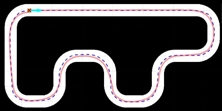
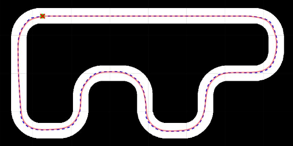
The trained agent completes the three circuits in the simulator. The image shown below is the result of DDPG trajectory (red) at circuit 2.
6.2 Simulator: classical algorithms
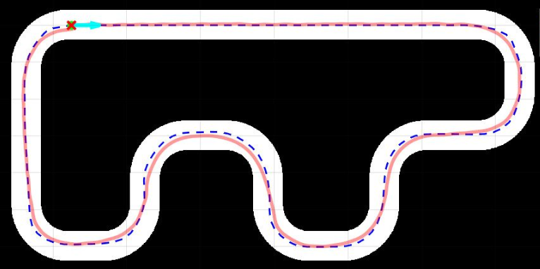
MPC, LQR and Pure Pursuit follow the same trajectory on the same circuit.
6.3 Simulator: comparison
These are the metrics for circuit 2: lap time (s), Mean Lateral Error (MLE) and Maximum Lateral Error (MAX) with respect to the centerline, and Lateral Jerk (LATJ) which measures how smooth are the lateral accelerations (the smaller the number, the less nervous the robot is).
Reference trajectory: centerline
| Time (s) | MLE (cm) | MAX (cm) | LATJ (m/s³) | |
|---|---|---|---|---|
| DDPG | 71.09 | 5.7 | 18.5 | 0.85 |
| PP | 72.78 | 2.2 | 6.7 | 0.17 |
| LQR | 72.40 | 3.9 | 10.2 | 1.48 |
| MPC | 72.45 | 2.0 | 6.5 | 0.39 |
Reference trajectory: optimized racing line (classical controllers)
| Time (s) | MLE (cm) | MAX (cm) | LATJ (m/s³) | |
|---|---|---|---|---|
| PP | 71.69 | 2.1 | 4.9 | 0.09 |
| LQR | 71.30 | 3.7 | 9.6 | 1.33 |
| MPC | 71.32 | 1.8 | 6.3 | 0.38 |
What the numbers say:
- DDPG has the fastest lap, 71.09 s. That is 1.3 to 1.7 seconds (about 2%) faster than the classical controllers following the centerline. This is due to the fact that the DDPG agent learnt how not to follow the centerline in a strict way; instead, it discovered that sacrificing lateral error was the best way to reduce total lap time. In other words the agent found the racing line which traces smoother and less pronounced curves improving lap time.
- The optimized racing line helps the classical controllers a lot. Each of them gains about 1.1 seconds, meaning that the mathematically found racing line works. Now, the gap to DDPG shrinks to +0.2 (LQR) to +0.6 seconds (PurePursuit). DDPG own racing line is still faster!
- DDPG pays in precision and smoothness. Its lateral jerk is higher than that of Pure Pursuit and MPC, although LQR is rougher still. Part of that error may come from the agent choosing its own line instead of the centerline, which creates little oscillations.
6.4 Results: real robot
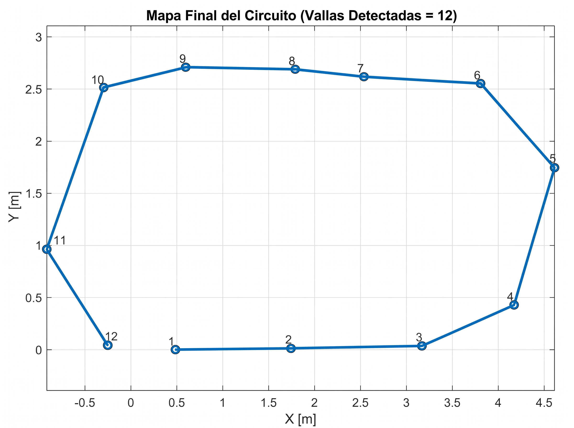
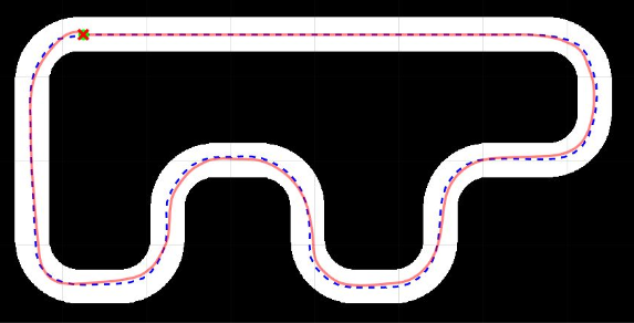
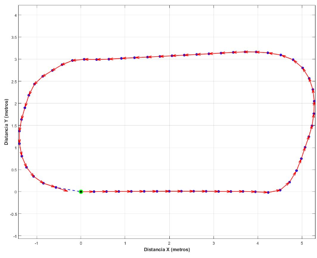
The last step was to take all four controllers to the physical TurtleBot 4 Lite, on a very simple rectangular circuit. The circuit waypoints were obtained by the ArUco markers and later optimized with the Spline algorithm, which is shown in the images below.
| Time (s) | MLE (cm) | MAX (cm) | LATJ (m/s³) | |
|---|---|---|---|---|
| DDPG | 57.70 | 10 | 22 | 0.94 |
| PP | 57.40 | 3.7 | 10 | 0.11 |
| LQR | 57.81 | 6.8 | 18 | 0.30 |
| MPC | 57.41 | 3 | 8.6 | 0.16 |
The advantage seen in simulation disappears here:
- All four lap times fall within 0.4 seconds of each other, and Pure Pursuit and MPC are slightly faster than DDPG.
- DDPG is clearly the least precise and least smooth, whit the highest lateral jerk which caused bigger oscillations. Its maximum error, 22 cm, is very close to the 23cm limit used to end the training episodes. This means that the agent tried to find faster speeds while cutting corners by leaning towards the track limits (which would have caused penalties during the training). Despite these drawbacks, DDPG lap times are still very close to the long-established controllers, so we shouldn’t take anything away from it.
I attribute the difference to the sim-to-real gap:
- The physical environment is not ideal like the simulator.
- The odometry estimate is very noisy.
- The wheels slip and have real friction with the floor.
- There is computational latency.
7. Conclusions
- Planning: I planned and optimized trajectories from waypoints for several circuits.
- RL training: I trained a DDPG agent that follows the different trajectories while maximizing speed, and that finds its own racing line, cutting corners naturally without relying on a precomputed optimization.
- Simulator: I compared the classical controllers with the RL agent. The agent got the best lap time, with a small margin, at the cost of tracking precision.
- Real tests: I deployed all the algorithms on the physical TurtleBot 4, where the classical controllers turned out to be more robust than the agent.
My takeaway: a reinforcement learning agent, with no precomputed racing line, beat in lap time the classical controllers that have been used for decades, and it found a good racing line all by itself. It was faster than Pure Pursuit, LQR and MPC following the centerline (by 1.3 to 1.7 seconds on a 71-second lap), and it stayed ahead of them even when they were given the optimized racing line. In racing, where results are decided by fractions of a second, that is a result I am proud of.
What remains is the step from simulation to the real world. On the real robot the agent oscillates more than the classical controllers, which costs it precision. My hypothesis is that closing the sim-to-real gap and smoothing those oscillations (domain randomization is the first thing I would try) is what separates this agent from a truly powerful racing controller.
Resources
If you are interested in the complete technical documentation, control models, or implementation details: